Mastering Twin-Y-Axis Line Charts in Excel: A Complete Information
Associated Articles: Mastering Twin-Y-Axis Line Charts in Excel: A Complete Information
Introduction
With nice pleasure, we are going to discover the intriguing matter associated to Mastering Twin-Y-Axis Line Charts in Excel: A Complete Information. Let’s weave fascinating data and provide recent views to the readers.
Desk of Content material
Mastering Twin-Y-Axis Line Charts in Excel: A Complete Information

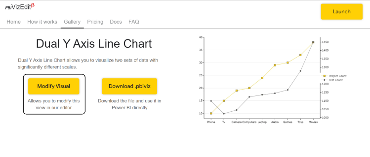
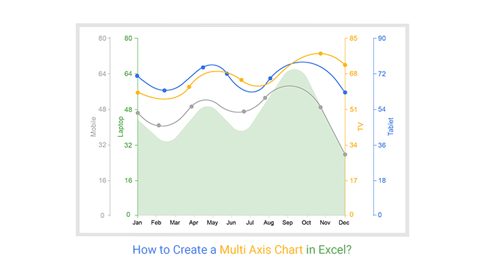
Line charts are a staple of knowledge visualization, successfully showcasing tendencies and adjustments over time. Nonetheless, when your information entails two distinct metrics with vastly totally different scales, a single Y-axis can result in misinterpretations or an unclear visualization. That is the place the facility of dual-Y-axis line charts comes into play. This complete information will stroll you thru creating, customizing, and decoding dual-Y-axis line charts in Excel, equipping you with the abilities to successfully talk complicated information relationships.
Understanding the Want for Twin Y-Axes
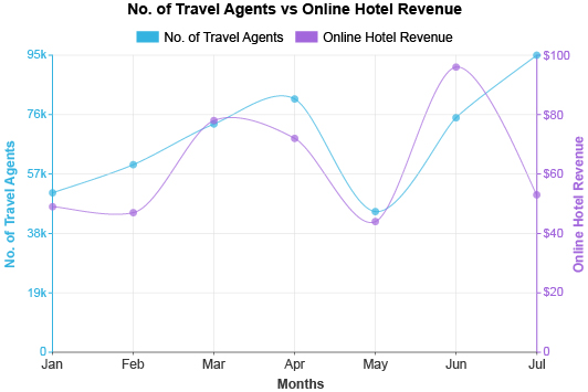
Think about you are monitoring web site site visitors (measured in hundreds of tourists) and common order worth (measured in {dollars}). Plotting each on a single Y-axis would both severely compress the web site site visitors information, making it virtually invisible, or drastically exaggerate the fluctuations in common order worth, making the adjustments seem much more important than they really are. A dual-Y-axis chart solves this drawback by assigning every metric its personal Y-axis, permitting each to be clearly visualized and in contrast throughout the identical chart.
Step-by-Step Information to Making a Twin-Y-Axis Line Chart in Excel
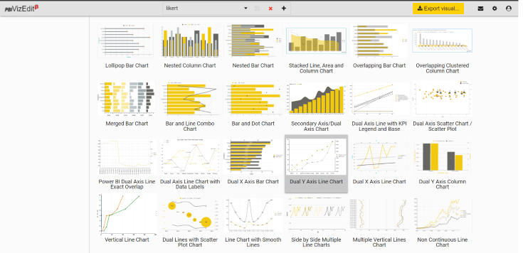
Whereas Excel does not instantly provide a "dual-Y-axis" chart sort, we will cleverly leverage its options to realize this. The method entails creating two separate line charts after which cleverly combining them. This is an in depth walkthrough:
1. Making ready Your Knowledge:
-
Set up your information: Guarantee your information is neatly organized in a spreadsheet. You will want at the least three columns: one for the X-axis (normally time, dates, or classes), and two for the Y-axis values (your two distinct metrics).
-
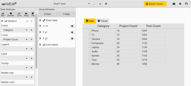
Instance Knowledge: Let’s assume you are monitoring web site visits and gross sales income over six months:
| Month | Web site Visits (Hundreds) | Gross sales Income ($) |
|---|---|---|
| January | 10 | 5000 |
| February | 12 | 6000 |
| March | 15 | 7500 |
| April | 18 | 8000 |
| Could | 20 | 9000 |
| June | 22 | 10000 |
2. Creating the First Line Chart:
- Choose your information: Choose the info to your first metric (e.g., Month and Web site Visits). Be certain to incorporate the header row.
- Insert a line chart: Go to the "Insert" tab and select the "Line" chart sort. Choose the primary line chart possibility (normally a easy 2D line chart). It will create a chart exhibiting web site visits over time.
3. Creating the Second Line Chart:
- Choose your information: Choose the info to your second metric (e.g., Month and Gross sales Income). Once more, embrace the header row.
- Insert a second line chart: Repeat step 2 to create a second line chart exhibiting gross sales income over time.
4. Combining the Charts (The Key Step):
- Choose the second chart: Click on on the second chart (Gross sales Income chart) to pick out it.
- Copy the chart: Press Ctrl+C (or Cmd+C on a Mac) to repeat the chart.
- Choose the primary chart: Click on on the primary chart (Web site Visits chart).
- Paste the chart: Proper-click throughout the first chart and select "Paste Particular."
- Select "Paste as Image": Within the Paste Particular dialog field, choose "Paste as Image" and click on "OK". This pastes the second chart as a picture onto the primary chart.
5. Adjusting the Second Chart’s Place and Dimension:
- Resize and reposition: Use the handles across the pasted picture of the second chart to resize it and completely align it with the primary chart. Be certain the X-axes align completely.
6. Including the Second Y-Axis:
- Choose the pasted chart: Click on on the pasted (Gross sales Income) chart picture.
- Format the chart space: Proper-click on the pasted chart and choose "Format Chart Space."
- Choose "Collection Choices": Within the Format Chart Space pane, search for "Collection Choices" (it is perhaps underneath "Chart Choices").
- Change the plot space: Below the "Collection Choices," find "Plot Collection On" and choose "Secondary Axis." It will routinely transfer the Gross sales Income line to a brand new Y-axis on the best aspect of the chart.
7. Customizing Your Chart:
- Axis Labels: Guarantee each Y-axes have clear and descriptive labels indicating the items (hundreds for web site visits, {dollars} for gross sales income).
- **Chart

Closure
Thus, we hope this text has offered beneficial insights into Mastering Twin-Y-Axis Line Charts in Excel: A Complete Information. We hope you discover this text informative and helpful. See you in our subsequent article!